How to sample from a hazard function
When you develop new methods, it’s important to test them on simulated data. Recently I’ve been developing some survival analysis methods and found myself needing to simulate survival data sets with arbitrary hazard functions. I searched and searched and couldn’t find a good way to do it, so I thought I’d share my solution here.
Still alive?
Survival analysis is the part of statistics that deals with waiting. It is named for that special kind of waiting in which we all must participate, but it is applicable to any kind of waiting for something to happen. I like to use it at the airport, for example. The core object in survival analysis is the survival function, which gives the probability that you will still be waiting (e.g., still alive) as a function of time. The hazard function is the negative time derivative of the survival function normalized by the survival function,
or, more intuitively, it is the instantaneous rate at which events (such as death) occur among the remaining survivors.
Sampling from the hazard function means drawing random numbers from the distribution that that hazard function implies. Fortunately, the survival function is related to the CDF by
and to the hazard function by
It is therefore possible, in principle, to compute the CDF from nothing but the hazard function. Knowing the CDF, it is possible to compute the inverse of the CDF, and it is this fact which I exploit.
Inverse transform sampling
The probability integral transform (PIT) is a super useful thing to know about. It’s used in multiple statistical methods and is the core of copula theory. I’ve asked people about it in interviews before. Anyway, the PIT says that for any random variable \(X\) with CDF \(F_{X}\), the random variable
is distributed Uniform(0,1). Super simple. If you want to sample from the distribution with CDF \(F_{X}\) and you know how to sample from the uniform distribution, all you need to do is take the inverse transform of your uniform sample! Therefore, if I can get an inverse CDF from my hazard function, then I can sample using inverse transform sampling.
Putting the pieces together
The key steps are as follows:
- Draw a number, \(u\), from the Uniform(0,1) distribution
- Use some numerical solver to solve \(u=F\left(t\right)\)
- The solution, \(t\), from step 2 is drawn from the desired distribution
It is step 2 that’s tricky, of course. All I have is the hazard function, and I need to find the inverse of the CDF. I used a bisection solution strategy to solve the equation in 2. To evaluate the CDF at each step of the bisection search, I used scipy.integrate.quad to numerically integrate the hazard function, then exploited the relationship between cumulative hazard and CDF. The full code is in this gist.
Demonstration
In the code below I sample survival times from the distribution implied by the hazard function
Check it out.
import numpy
from samplers import HazardSampler
# Set a random seed and sample size
numpy.random.seed(1)
m = 1000
# Use this totally crazy hazard function
hazard = lambda t: numpy.exp(numpy.sin(t) - 2.0)
# Sample failure times from the hazard function
sampler = HazardSampler(hazard)
failure_times = numpy.array([sampler.draw() for _ in range(m)])
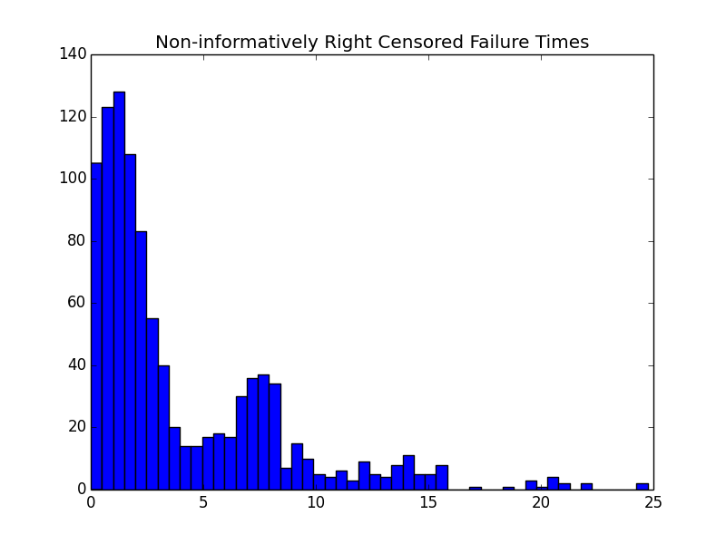
# Apply some non-informative right censoring, just to demonstrate how it's done
censor_times = numpy.random.uniform(0.0, 25.0, size=m)
y = numpy.minimum(failure_times, censor_times)
c = 1.0 * (censor_times > failure_times
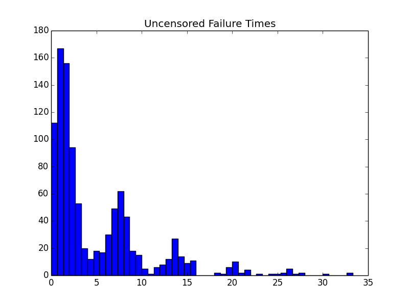
Now let’s make some plots to see how it looks. First I’ll make histograms of the uncensored and censored survival times. Then I’ll compare the true survival function to an estimate based on the uncensored sample.
# Make some plots of the simulated data
from matplotlib import pyplot
from statsmodels.distributions import ECDF
# Plot a histogram of failure times from this hazard function
pyplot.hist(failure_times, bins=50)
pyplot.title('Uncensored Failure Times')
pyplot.savefig('uncensored_hist.png')
pyplot.show()
# Plot a histogram of censored failure times from this hazard function
pyplot.hist(y, bins=50)
pyplot.title('Non-informatively Right Censored Failure Times')
pyplot.savefig('censored_hist.png')
pyplot.show()
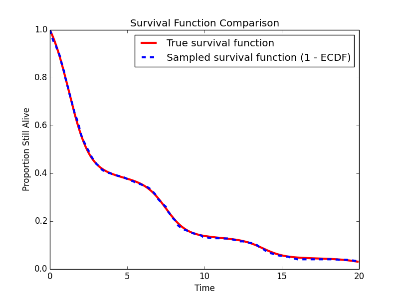
# Plot the empirical survival function (based on the censored sample) against the actual survival function
t = numpy.arange(0,20.0,.1)
S = numpy.array([sampler.survival_function(t[i]) for i in range(len(t))])
S_hat = 1.0 - ECDF(failure_times)(t)
pyplot.figure()
pyplot.title('Survival Function Comparison')
pyplot.plot(t, S, 'r', lw=3, label='True survival function')
pyplot.plot(t, S_hat, 'b--', lw=3, label='Sampled survival function (1 - ECDF)')
pyplot.legend()
pyplot.xlabel('Time')
pyplot.ylabel('Proportion Still Alive')
pyplot.savefig('survival_comp.png')
pyplot.show()
The resulting histograms look about how you’d expect for this weird hazard function.
The sample estimated survival function matches well with the actual survival function.
Final thoughts
This algorithm is kind of slow, since it involves repeated numerical integration. Furthermore, my implementation is not as efficient as it could be. For example, I could do most of the numerical integration up front instead of on demand. I also do the root finding in pure Python. But, at least now I can draw samples from any hazard function I want! For my purposes the slowness is not such a big deal, as I only need to simulate data sets to test my hazard regression methods. Once I have the sample, I simply put it in a file and use it as needed. If you wanted to do this as part of some kind of monte carlo algorithm or something, you might need to write a more efficient implementation. I would estimate 100-1000x speedup is possible with a lot of effort.
Follow up
Apparently I should have searched harder, because it looks like there is actually an R package that does almost exactly what I wanted. I haven’t looked in detail, but it appears to also use an inversion-based method and I think handles arbitrary hazard functions.